
Bradley Gram-Hansen
Senior Applied Scientist Apple !
Doctorate from the University of Oxford in AI & Machine Learning.
The beginners guide to Hamiltonian Monte Carlo
In this post I will go through a powerful Markov Chain Monte Carlo (MCMC) algorithm called Hamiltonian Monte Carlo (HMC) (MC’s be in da house) and demonstrate how to implement the algorithm within the pytorch framework.
Let us start with a super nice gif demonstrating the conservation of momentum in action:

Why is momentum important?
Well, it makes things move. It gives things the spice of life and so when we have a particle, a sample and want it to explore the space
we need to make it move.
But, we want it to move efficiently around the space that we wish to explore.
It turns out that this Irish guy named Hamilton, the guy behind the Hamiltonian, found a really cool way of representing such systems so that paths that explore the space efficiently naturally pop out from the representation.
Hamilton showed that we can describe any mechanical system with just 2 variables,
or 2 degrees of freedom , represented by position \(q\) and momentum \(p\).
The Phase Space
Is just a fancy coordinate system that is defined in terms of position and momentum, so when we explore trajectories in the phase space, we explore contours of energy, that is the phase (angle with respect to position and momentum) changes in phase space! Here is an example phase space:
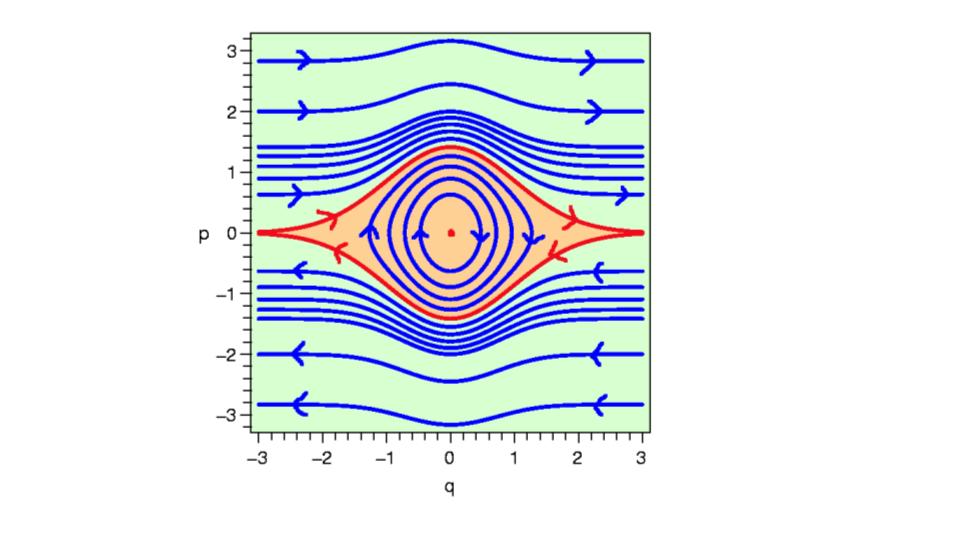
The red inner regions represent where the motion is stable, i.e, we have energy preserving trajectories. Take note of this, it is important. In fact, it is integral for why HMC works so well in high-dimensions. It relates to something called symplectic geometries, which essentially have lots of nice mathematically properties that just so happen to be the exact features we require for certain dynamical systems. #ConspiracyTheory. Because they preserve energy, we can define an MCMC strategy in which the chance of accepting a particle, sample is high, by defining the acceptance criteria in terms of the total energy on these paths!
The regions outside of this red region are non-energy preserving - this is not gouda (I know my cheeses) for our MCMC algorithm, because this would lead to low-acceptance rates, thus our algorithm would be computationally inefficient at exploring the space we are exploring! Hence, we want to construct a system that is energy preserving. #ConservationOfEnergy
Thankfully, Hamilton provided us with a way to easily find these trajectories!
The Hamiltonian
The Hamiltonian of a physical system is defined completely with respect to the position \(q\) and \(p\) momentum variables and defines the total energy of the system on a particular trajectory for a given \(q\) and \(p\), the circles on the phase space diagram above.
The Hamiltonian is the Legendre transform of the Lagrangian and gives us the total energy in the system. All you need to know about the Lagrangian is that the Lagrangian was just another representation for describing the energy in dynamical systems, which itself was an extension of Newtonian formalism, it is basically a function of kinetic energy minus potential energy. It is defined as follows: \begin{equation} \label{one}\tag{1} H(q,p) = \sum_{i = 1}^{d}\dot{q}_i p_i - L(q, \dot{q}(q, p)) \end{equation} where \(d\) is the system dimensions, and so the full state space has \(2d\) dimensions (as we require 2 variables to describe the dynamics in each dimension). The \(\dot{}\) here corresponds to a derivative with respect to time, i.e \(\dot{q} = \frac{dq}{dt}\).
Thus, for simplicity, if we set \(d = 1\) we can derive the Hamiltonian equations as follows:
\begin{equation}
\label{hameq1}\tag{2}
\frac{\partial H}{\partial p} = \dot{q} + p\frac{\partial \dot{q}}{\partial p} - \frac{\partial L}{\partial \dot{q}}\frac{\partial \dot{q}}{\partial p} = \dot{q}
\end{equation}
and
\begin{equation}
\label{hameq2}\tag{3}
\frac{\partial H}{\partial q} = p\frac{\partial \dot{q}}{\partial q} - \frac{\partial L}{\partial q} - \frac{\partial L}{\partial \dot{q}}\frac{\partial \dot{q}}{\partial q} = - \frac{\partial L}{\partial q}= -\dot{p}
\end{equation}
and the process is the same for more than one dimension, you just set \(d=n\) ;-). We can write \eqref{one} more succinctly as: \begin{equation} \label{hamreduced}\tag{4} H(q, p) = K(p) + U(q) \end{equation}
where \(K(p)\) represents our kinetic energy and \(U(q)\) is the potential energy. Equation \(\eqref{hamreduced}\) comes from the following: \(L(q, \dot{q}(q, p)) = \frac{1}{2}p\dot{q} - U(q)\) as momentum \(p = m\dot{q}\) and we would add a summation to this to represent each dimension.
I hope that you are beginning to feel all that potential at your finger tips - well almost - bad joke I know…

Hamiltonian Monte Carlo
Within the HMC MCMC framework the positions, \(q\), are the variables of interest and for each position variable we have to create a fictitious momentum, \(p\). For compactness let \(z = (q,p)\). The potential energy \(U(q)\) will be the minus of the log of the probability density for the distribution of the position variables we wish to sample, plus any constant that is convenient. The kinetic energy will represents the dynamics of our variables, for which a popular form of \(K(p) = \frac{p^{T} M^{-1} p}{2}\), where \(M\) is symmetric, positive definite and typically diagonal. This form of \(K(p)\) corresponds to a minus the log probability of the zero mean Gaussian distribution with covariance matrix \(M\), more on the choice of kinetic energy later. For this choice of kinetic energy we can write the Hamiltonian equations as follows:
$$\begin{align} \dot{q} &= M^{-1}p \label{position}\tag{5}\\ \dot{p} &= -\frac{\partial U}{\partial q} \label{momentum}\tag{6} \end{align}$$
It should be noted that \(M\) can take on different properties, which can effect the way that we explore the space in numerous ways. More on this in another blog post, as it gets a little complicated.
The Canonical Distribution
To view the Hamiltonian in terms of probabilities, we use the concept of the canonical distribution from Statistical mechanics to construct our probability density function - it is a density because we define our space to be continuous. Thus, the distribution that we wish to sample from can be related to the potential energy via the canonical distribution as: \begin{equation} \label{canonical}\tag{7} P(z) = \frac{1}{Z}\exp\left(\frac{-E(z)}{T}\right) \end{equation} As the Hamiltonian is just an energy function we may can insert \eqref{hamreduced} into our canonical distribution \eqref{canonical}, which gives us the joint density: \begin{equation} \tag{8} P(q,p) = \frac{1}{Z}\exp(-U(q))\exp(-K(p)) \end{equation}
where \(T = 1\) is fixed. And so we can now very easily get to our target distribution \(p(q)\), which is dependent on our choice of potential \(U(q)\), as this expression factorizes into two independent probability distributions. We characterise the posterior distribution for the model parameters using the potential energy function: \begin{equation} \tag{9} U(q) = -\log[p(q)p(q|D)] \end{equation} where \(p(q)\) is the prior distribution, and \(p(q|D)\) is the likelihood of the given data \(D\).
Solving Hamilton’s Equations
In order to solve the set of differential equations generated from Hamilton’s formalism we need to integrate. If the potential function (joint density in the MCMC (Bayesian) framework) is well understood, then it maybe possible to solve Hamilton’s equations analytically. However, in many instances in both the physical and statistical setting you have functions that generate integrals that are impossible to solve analytically using known techniques. A resolution to this is to employ numerical methods, which produce an approximation that is close to the true value. However, to implement a numerical solver requires us to discretize Hamilton’s equations which induces errors #Boo!
Errors of Numerical Solvers
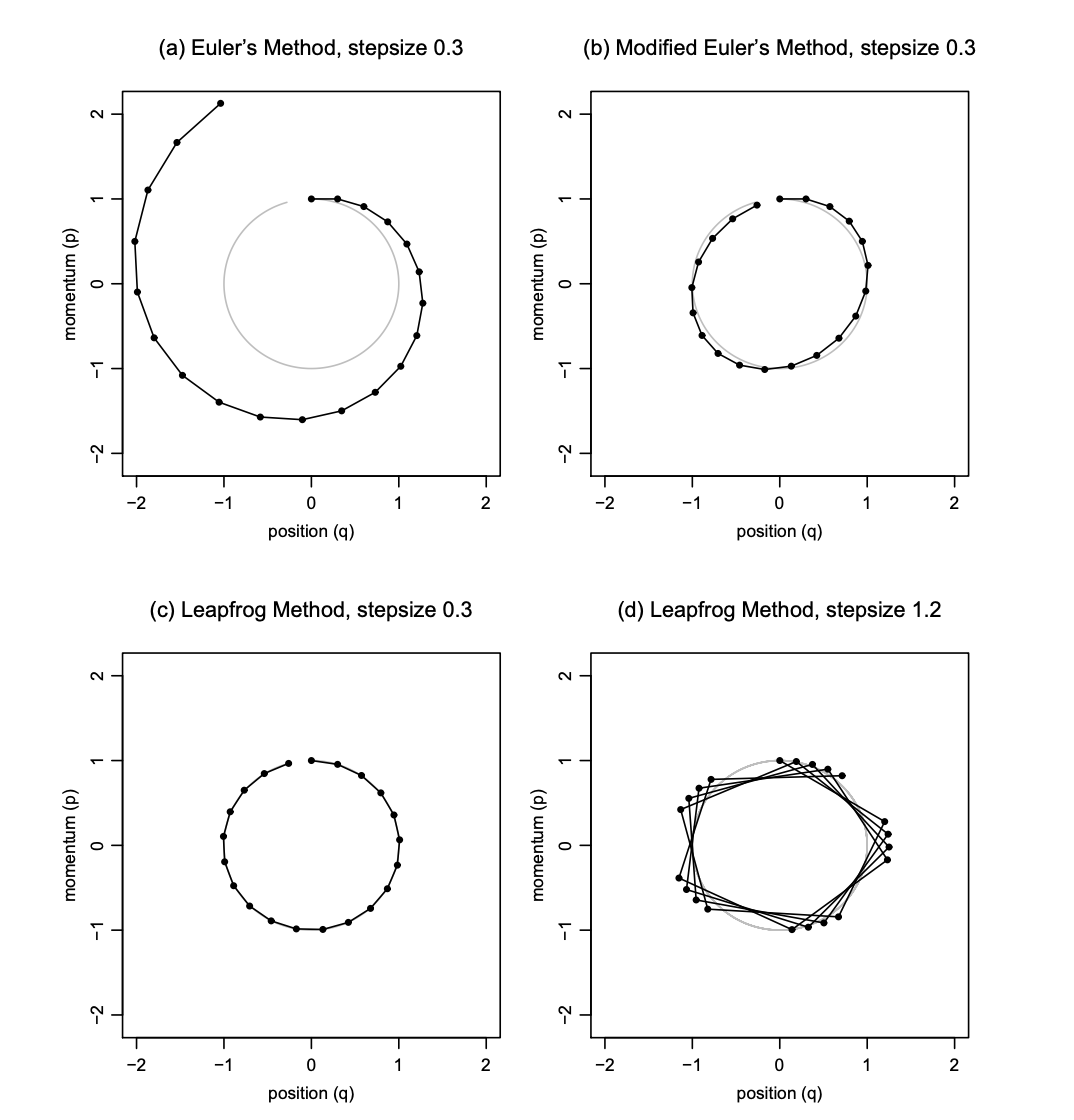
One could employ Euler’s method for solving a series of differential equations, however, it has less than desirable properties in regards to the local and global errors incurred in the approximation #OhNo. Where local error, is the error after one step and global error, is the error after simulating for some fixed time interval. A more optimal integrator is the Leapfrog integrator, that has a local error of \(\mathcal{O}(\epsilon^{2})\) and a global error of \(\mathcal{O}(\epsilon^{3})\) #Yay!.
Here is a nice figure, directly lifted from [1] Radford Neal’s paper, showing how trajectories diverge between the Euler and Leapfrog integrators.
The Leapfrog Integrator
Both the Leapfrog integrator and the Euler integrator are part of a class of symplectic integrators, i.e they are volume preserving. Both could be used for HMC, but as the Leapfrog integrator has significantly lower local and global errors it has become the integrator of choice. The integrator first starts with a particle at \(t = 0\) and then evaluates the updated dynamics, subject to the form of the Hamiltonian, equation \(\eqref{hamreduced}\), at subsequent times \(t + \epsilon , \ldots, t + n\epsilon\), where \(\epsilon\) is the stepsize in which we increase our dynamical moves and \(n\) is the number of time steps to simulate the dynamics for.
$$\begin{align} p_{i}(t + \frac{\epsilon}{2}) &= p_{i}(t) - \left(\frac{\epsilon}{2}\right)\frac{\partial U(q(t))}{\partial q_{i}} \tag{10} \\ q_{i}(t + \epsilon) &= q_{i}(t) + \epsilon\frac{\partial K(p(t + \frac{\epsilon}{2}))}{dp_{i}} \tag{11}\\ p_{i}(t + \epsilon) &= p_{i}(t + \frac{\epsilon}{2}) - \left(\frac{\epsilon}{2}\right)\frac{\partial U}{\partial x_{i}} \tag{12}\\ \end{align}$$
For the usual choice of kinetic energy, we have \(\frac{\partial K(p + \frac{\epsilon}{2})}{dp_{i}} = \frac{p_{i}(t + \frac{\epsilon}{2})}{m_{i}}\), but it doesn’t have to be this kinetic energy!
Some initial points to notice
HMC can only be used to sample from continuous distributions on \(\mathbb{R}^{d}\) for which a density function can be evaluated. We must be able to compute the partial derivative of the log of the density function. The derivatives must exists at the points at which they are evaluated. HMC samples from the canonical distribution for \(q\) and \(p\). \(q\) has the distribution of interest as specified by the potential \(U(q)\). The distribution of the \(p\)’s can be chosen by us and are independent of the \(q\)’s. The \(p\) components are specified to be independent, with component \(p_{i}\) having variance \(m_{i}\). The kinetic energy \(K(p) = \sum_{i =1}^{d}\frac{p_{i}^{2}}{2m_{i}}(q(t + \epsilon))\). It should be noted that you can use different kinetic energies and these will all have varying effects, see here for more details. The standard kinetic energy actually has a direct link to the Gaussian distribution, and can be seen as average energy over all states. This is linked to the Boltzmann distribution in statistical physics, see here for more details.
The Hamilton Monte Carlo Algorithm
So we are nearly there, it is time for the final part. Each iteration of the HMC algorithm has two steps.
- The first changes only the momentum (We sample \(p \sim N(0,1)\) (in n-dim we sample from \(MultiNormal(0, M)\))).
- The second may change both position and momentum (We apply the leapfrog integrator and then decided whether or not to accept).
In the first step, new values for the momentum variables are randomly drawn from their Gaussian distribution, independently of the current values of the position variables. For the kinetic energy, in \(d\)-dimensions, each momentum variable is independent, but only if we choose a covariance matrix \(M\) such that this is the case #ItDoesntHaveToBe. In the second step, a Metropolis update is performed, using Hamiltonian dynamics to propose a new state. Starting with the current state, \((q, p)\), Hamiltonian dynamics is simulated for \(L\) steps using the Leapfrog method (or some other reversible method that preserves volume), with a stepsize of \(\epsilon\). Here, \(L\) and \(\epsilon\) are parameters of the algorithm, which need to be tuned to obtain good performance, see here for details on tuning. The momentum variables at the end of this \(L\)-step trajectory are then negated, giving a proposed state \((q^∗, p^∗)\). This proposed state is accepted as the next state of the Markov chain with probability: \begin{equation} \min[1, \exp(−H(q^∗, p^∗) + H(q, p)] = \min[1, exp(−U(q^*) + U(q) − K(p^∗) + K(p))] \end{equation}
So, you are definitely wondering, if the trajectories that this is simulating are energy preserving trajectories, why is the acceptance probability not always 1, because surely \(H(q^∗, p^∗) = H(q, p)\) ? Well spotted! This is because when we discretize Hamiltonian’s equations to solve them via our numerical solver errors are introduced. Thus, we may not always get an acceptance probability of 1. In fact, it may not be best to have an acceptance probability of 1, see here.
Here is an awesome visual of HMC in action from chi-feng’s github page:

The Hamiltonian Monte Carlo algorithm starts at a specified initial set of parameters \(q\), see code below. Then, for a given number of iterations, a new momentum vector is sampled and the current value of the parameter \(q\) is updated using the leapfrog integrator with discretization time \(\epsilon\) and number of steps \(L\) according to the Hamiltonian dynamics. Then a Metropolis acceptance step is applied, and a decision is made whether to update to the new state \((q^∗,p^*)\) or keep the existing state, see code below.
How to Implement HMC in a System
I’m going slightly exaggerate some aspects of the code, so that it is clear how one can implement HMC more generally and if needed, for research purposes, add your own HMC flavor. Disclaimer: This code is not optimised for speed, it is here for readability and clarity.
I should also note, that once Pytorch 0.4 has been released, all Variable statements can be replaced with torch.tensor(data=...) and if you want the gradients of those objects, then you do torch.tensor(data=... , dtype=..., requires_grad=True)
We are going to use a helper function for now called VariableCast(), for Pytorch v0.3 and lower, which handles this automatically:
    import torch
    from torch.autograd.variable import Variable
    def VariableCast(value, grad = False):
        '''
        Casts an input to torch Variable object, with gradients either False or True.
        input
        -----
        value - Type: scalar, Variable object, torch.Tensor, numpy ndarray
        grad  - Type: bool . If true then we require the gradient of that object
        output
        ------
        torch.autograd.variable.Variable object
        '''
        if value is None:
            return None
        elif isinstance(value, Variable):
            return value
        elif torch.is_tensor(value):
            return Variable(value, requires_grad = grad)
        elif isinstance(value, np.ndarray):
            tensor = torch.from_numpy(value).float()
            return Variable(tensor, requires_grad = grad)
        elif isinstance(value,list):
            return Variable(torch.FloatTensor(value), requires_grad=grad)
        else:
            return Variable(torch.FloatTensor([value]), requires_grad = grad)
The Integrator
    #!/usr/bin/env python3
    # -*- coding: utf-8 -*-
    import torch
    import numpy as np
    from kinetic import Kinetic
    from torch.autograd import Variable

    class Integrator():

        def __init__(self, potential, min_step, max_step, max_traj, min_traj):
            self.potential = potential
            if min_step is None:
                self.min_step = np.random.uniform(0.01, 0.07)
            else:
                self.min_step = min_step
            if max_step is None:
                self.max_step = np.random.uniform(0.07, 0.18)
            else:
                self.max_step = max_step
            if max_traj is None:
                self.max_traj = np.random.uniform(18, 25)
            else:
                self.max_traj = max_traj
            if min_traj is None:
                self.min_traj = np.random.uniform(1, 18)
            else:
                self.min_traj = min_traj

        def generate_new_step_traj(self):
            ''' Generates a new step adn trajectory size  '''
            step_size = np.random.uniform(self.min_step, self.max_step)
            traj_size = int(np.random.uniform(self.min_traj, self.max_traj))
            return step_size, traj_size


        def leapfrog(self, p_init, q, grad_init):
            '''Performs the leapfrog steps of the HMC for the specified trajectory
            length, given by num_steps
            Parameters
            ----------
                values_init
                p_init
                grad_init     - Description: contains the initial gradients of the joint w.r.t parameters.

            Outputs
            -------
                q -    Description: proposed new q
                p      -    Description: proposed new auxillary momentum
            '''
            step_size, traj_size = self.generate_new_step_traj()
            values_init = q
            self.kinetic = Kinetic(p_init)
            # Start by updating the momentum a half-step and q by a full step
            p = p_init + 0.5 * step_size * grad_init
            q = values_init + step_size * self.kinetic.gauss_ke(p, grad=True)
            for i in range(traj_size - 1):
                # range equiv to [2:nsteps] as we have already performed the first step
                # update momentum
                p = p + step_size * self.potential.eval(q, grad=True)
                # update q
                q = q + step_size * self.kinetic.gauss_ke(p, grad=True)

            # Do a final update of the momentum for a half step
            p = p + 0.5 * step_size * self.potential.eval(q, grad=True)

            # return new proposal state
            return q, p
Kinetic Energy
    from core import VariableCast
    import torch
    from torch.autograd import Variable
    class Kinetic():
        ''' A basic class that implements kinetic energies and computes gradients
        Methods
        -------
        gauss_ke          : Returns KE gauss
        laplace_ke        : Returns KE laplace

        Attributes
        ----------
        p    - Type       : torch.Tensor, torch.autograd.Variable,nparray
            Size       : [1, ... , N]
            Description: Vector of current momentum

        M    - Type       : torch.Tensor, torch.autograd.Variable, nparray
            Size       : \mathbb{R}^{N \times N}
            Description: The mass matrix, defaults to identity.

        '''
        def __init__(self, p, M = None):

            if M is not None:
                if isinstance(M, Variable):
                    self.M  = VariableCast(torch.inverse(M.data))
                else:
                    self.M  = VariableCast(torch.inverse(M))
            else:
                self.M  = VariableCast(torch.eye(p.size()[0])) # inverse of identity is identity


        def gauss_ke(self,p, grad = False):
            '''' (p dot p) / 2 and Mass matrix M = \mathbb{I}_{dim,dim}'''
            self.p = VariableCast(p)
            P = Variable(self.p.data, requires_grad=True)
            K = 0.5 * P.t().mm(self.M).mm(P)

            if grad:
                return self.ke_gradients(P, K)
            else:
                return K
        def laplace_ke(self, p, grad = False):
            self.p = VariableCast(p)
            P = Variable(self.p.data, requires_grad=True)
            K = torch.sign(P).mm(self.M)
            if grad:
                return self.ke_gradients(P, K)
            else:
                return K
        def ke_gradients(self, P, K):
            return torch.autograd.grad([K], [P])[0]
Potential Energy
Step 1
Automatically calculating the gradients for an arbitrary function might sound difficult, but with any auto differentiation framework this is actually quite trivial.
In Pytorch we can do the following:
    def _grad_logp(self, logp, values):
        """
        Returns the gradient of the log pdf, with respect for
        each parameter

        Parameters
        ----------
        logjoint       - The density function
        values         - All parameters for which you need gradients.

        :return: torch.autograd.Variable
        """

        gradient_of_param = torch.autograd.grad(outputs=logp, inputs=values, retain_graph=True)[0]
        return gradient_of_param
Metropolis Step
    import torch
    from torch.autograd import Variable
    from Utils.kinetic import Kinetic

    class Metropolis():

        def __init__(self, potential, integrator, M):
            self.potential  = potential
            self.integrator = integrator
            self.M          = M
            self.count      = 0

        def sample_momentum(self,values):
            assert(isinstance(values, Variable))
            return Variable(torch.randn(values.data.size()))

        def hamiltonian(self, logjoint, p):
            """Computes the Hamiltonian  given the current postion and momentum
            H = U(q) + K(p)
            U is the potential energy and is = -log_posterior(q)
            Parameters
            ----------
            logjoint    - Type:torch.autograd.Variable
                        Size: \mathbb{R}^{1 \times D}
            p           - Type: torch.Tensor.Variable
                        Size: \mathbb{R}^{1 \times D}.
                        Description: Auxiliary momentum
            log_potential :Function from state to position to 'energy'= -log_posterior

            Returns
            -------
            hamitonian : float
            """
            T = self.kinetic.gauss_ke(p, grad=False)
            return -logjoint + T
        def acceptance(self, values_init, logjoint_init, grad_init):
            '''Returns the new accepted state

            Parameters
            ----------

            Output
            ------
            returns accepted or rejected proposal
            '''

            # generate initial momentum

            #### FLAG
            p_init = self.sample_momentum(values_init)
            # generate kinetic energy object.
            self.kinetic = Kinetic(p_init, self.M)
            # calc hamiltonian  on initial state
            orig = self.hamiltonian(logjoint_init, p_init)

            # generate proposals
            values, p = self.integrator.leapfrog(p_init, values_init, grad_init)

            # calculate new hamiltonian given current
            logjoint_prop, _ = self.potential.eval(values, grad=False)

            current = self.hamiltonian(logjoint_prop, p)
            alpha = torch.min(torch.exp(orig - current))
            # calculate acceptance probability
            if isinstance(alpha, Variable):
                p_accept = torch.min(torch.ones(1, 1), alpha.data)
            else:
                p_accept = torch.min(torch.ones(1, 1), alpha)
            # print(p_accept)
            if p_accept[0][0] > torch.Tensor(1, 1).uniform_()[0][0]:  # [0][0] dirty code to get integersr
                # Updates count globally for target acceptance rate
                # print('Debug : Accept')
                # print('Debug : Count ', self.count)
                self.count = self.count + 1
                return values, self.count
            else:
                # print('Debug : reject')
                return values_init, self.count
Tying Everything Together
    import torch
    import numpy as np
    import time
    import math
    from torch.autograd import Variable
    from Utils.integrator import Integrator
    from Utils.metropolis_step import Metropolis
    # np.random.seed(12345)
    # torch.manual_seed(12345)
    class HMCsampler():
        '''
        Notes:  the params from FOPPL graph will have to all be passed to - maybe
        Methods
        -------
        leapfrog_step - preforms the integrator step in HMC
        hamiltonian   - calculates the value of hamiltonian
        acceptance    - calculates the acceptance probability
        run_sampler

        Attributes
        ----------

        '''
        def __init__(self, program, burn_in= 100, n_samples= 20000, M= None,  min_step= None, max_step= None,\
                    min_traj= None, max_traj= None):
            self.burn_in    = burn_in
            self.n_samples  = n_samples
            self.M          = M
            self.potential  = program()
            self.integrator = Integrator(self.potential, min_step, max_step, \
                                        min_traj, max_traj)
            # self.dim        = dim

            # TO DO : Implement a adaptive step size tuning from HMC
            # TO DO : Have a desired target acceptance ratio
            # TO DO : Implement a adaptive trajectory size from HMC


        def run_sampler(self):
            ''' Runs the hmc internally for a number of samples and updates
            our parameters of interest internally
            Parameters
            ----------
            n_samples
            burn_in

            Output
            ----------
            A tensor of the number of required samples
            Acceptance rate
            '''
            print(' The sampler is now running')
            # In the future dim = # of variables will not be needed as Yuan will provide
            # that value in the program and it shall return the required dim.
            logjoint_init, values_init, grad_init, dim = self.potential.generate()
            metropolis   = Metropolis(self.potential, self.integrator, self.M)
            temp,count   = metropolis.acceptance(values_init, logjoint_init, grad_init)
            samples      = Variable(torch.zeros(self.n_samples,dim))
            samples[0]   = temp.data.t()


            # Then run for loop from 2:n_samples
            for i in range(self.n_samples-1):
                logjoint_init, grad_init = self.potential.eval(temp, grad_loop= True)
                temp, count = metropolis.acceptance(temp, logjoint_init, grad_init)
                samples[i + 1, :] = temp.data.t()
                # try:
                #     samples[i+1,:] = temp.data.t()
                # except RuntimeError:
                #     print(i)
                #     break
                # update parameters and draw new momentum
                if i == np.floor(self.n_samples/4) or i == np.floor(self.n_samples/2) or i == np.floor(3*self.n_samples/4):
                    print(' At interation {}'.format(i))

            # Basic summary statistics
            target_acceptance =  count / (self.n_samples)
            samples_reduced   = samples[self.burn_in:, :]
            mean = torch.mean(samples_reduced,dim=0, keepdim= True)
            print()
            print('****** EMPIRICAL MEAN/COV USING HMC ******')
            print('empirical mean : ', mean)
            print('Average acceptance rate is: ', target_acceptance)

            return samples,samples_reduced, mean
References
The canonical papers are: